Science
Our quantum gas microscope allows us to detect single atoms, opening the door to new directions for physics studies. First, we are interested in exploring atoms in a “bulk” gas using our microscope solely for readout. Large ensembles of atoms in a harmonic trap exhibit a wide range of phenomena spanning from superfluidity to vortex formation. Studying these ensembles microscopically offers the capability to probe observables not afforded by standard low-resolution imaging like short-range correlations. For future studies, we plan to extend these techniques to new regimes using spin-dependent potentials developed in previous studies on this experimental platform.
Imaging the thermal de Broglie wavelength
- In situ imaging of the thermal de Broglie wavelength in an ultracold Bose gas, Phys. Rev. Lett. (2025)
- Featured Physics Viewpoint
- Physics World article
Our first experiment with our microscope emulated the original Hanbury Brown and Twiss (HBT) experiment using ultracold atoms behaving as matter waves rather than photons. HBT observed a spatial correlation of the intensity fluctuations for light emitted from the distant star Sirius. These fluctuations represent an optical speckle pattern with a characteristic length scale of the optical wavelength $\lambda$ on the star’s surface. When light propagates from a distant star of radius $R$ to the earth at distance $D$, the speckle size is magnified to $\lambda D/R$, which HBT determined to be around $5~\mathrm{m}$ for Sirius. Matter waves have an equivalent speckle pattern with a characteristic grain size of the thermal de Broglie wavelength $\lambda_{\text{dB}} = h/\sqrt{2\pi m k_{B} T}$. Similar to light propagation, ballistic expansion of ultracold atoms magnifies the $\textit{in situ}$ correlation length in the far-field by $D/R$.
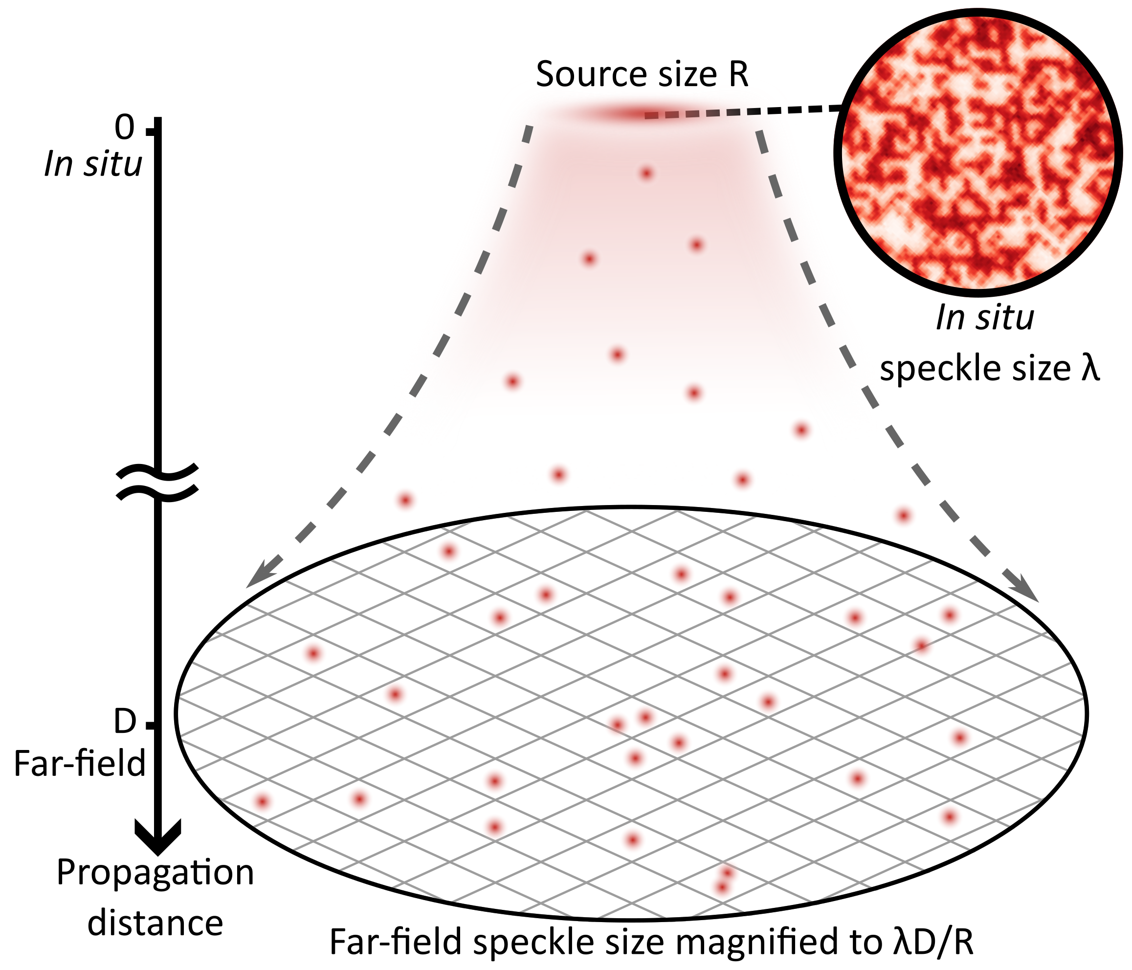
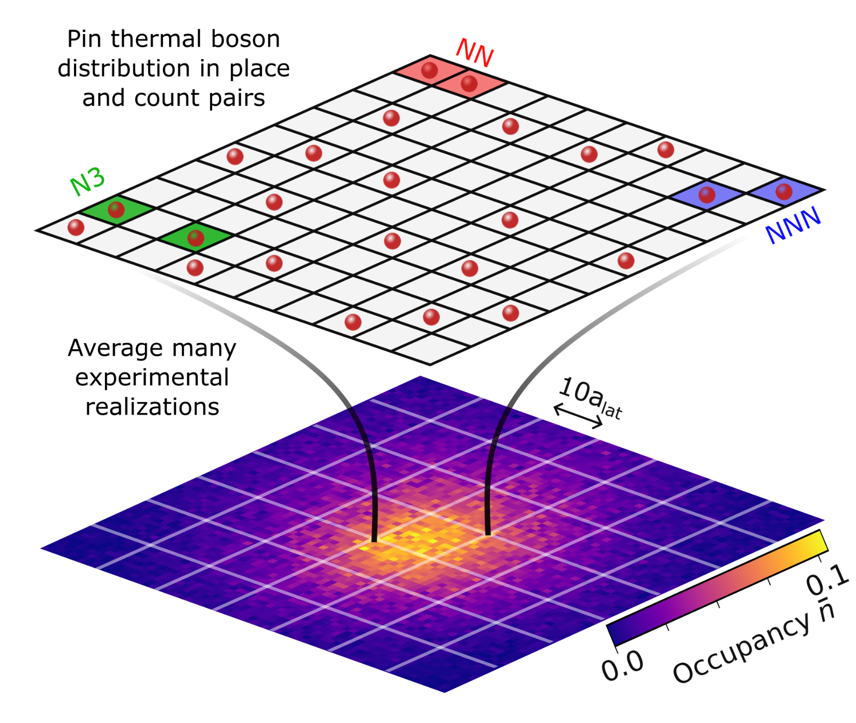
To detect this speckle pattern, we project the 2D Bose distribution onto a pinning lattice and reconstruct the site-by-site lattice occupation. To determine the bosonic enhancement, we count pairs of atoms separated by distance $r$ and determine the enhancement factor $g^{(2)}(r)$ over the classical distribution corresponding to fully distinguishable particles. On the lattice grid, we show the distance between three types of pairs, corresponding to the nearest-neighbor (NN, red), next-nearest-neighbor (NNN, blue), and third-nearest-neighbor (N3, green).
Next, we will extend these correlation studies to new confinement and interaction regimes.
Preparing our system around $T/T_{C}$, we observe a microscopic realization of the BEC phase transition.
Previously, we studyied the mapping between the Bose–Hubbard model with a spin degree of freedom and the $S = 1$ Heisenberg model. Have a look at our MIT wiki page for a complete list of previous publications.
The spin Mott insulator
- Preparation of the Spin-Mott State: A Spinful Mott Insulator of Repulsively Bound Pairs, Phys. Rev. Lett. 129, 093401 (2022)
Particles in a sufficiently deep lattice can be described by the Bose-Hubbard model. Here we assume they tunnel around with some rate $t$, and that they have an on-site interaction $U$. In our lab we’ve been studying what happens when there are two particles per site which are allowed to be in different spin states. We denote these by A and B, but really they’re just different hyperfine states of rubidium ($|F, m_F\rangle$). Things get interesting when they have a tunable interparticle interaction $U_{AB}$ (typically such that $0 \leq U_{AB} \leq U$). If we tune this all the way to zero, the energetically most favorable state is to have an A and a B particle on every site, this is the spin Mott insulator, and we studied it in the paper mentioned above.
When $U_{AB} = U$, the ground state is highly degenerate: it doesn’t matter what spin configuration you have anymore, because all energies are the same. On the way to that point, however, the AB state starts to ‘fluctuate,’ meaning it will undergo excursions to AA or BB. These fluctuations are highly correlated between neighbors - after all, they need to exchange particles - and this tate is called an XY ferromagnet. (Our lab was involved in a theory collaboration to explore the full phase diagram.)
In the lab we implement this using a spin-dependent lattice, which gives us control over the overlap of the atomic wave functions in the lattice. It allows us to tune $U_{AB}$. Below you can try so yourself - notice the fluctuations into paired states that arise as you approach perfect overlap.
A cartoon of the spin Mott insulator. Drag the wave functions to change their overlap.
Spin-1 out of equilibrium
- Tunable Single-Ion Anisotropy in Spin-1 Models Realized with Ultracold Atoms, Phys. Rev. Lett. 126, 163203 (2021)
We can use our the spin degree of freedom to mimic a $S = 1$ Heisenberg Hamiltonian. Under this transformation, the occupation states $|AA\rangle$, $|AB\rangle$ and $|BB\rangle$ are mapped onto $|S = 1, m_S\rangle$ states which we can abbreviate as $|\Downarrow\rangle$, $|\circ\rangle$, and $|\Uparrow\rangle$.
We have studied the behavior of this model in the presence of an anisotropy, i.e. a term in the Hamiltonian proportional to $(S_z)^2$. If this term is positive it favors populating the $|\circ\rangle$ state ($S_z = 0$), if it’s negative it favors $S_z = \pm 1$. We investigated the effect of this term by preparing all effective spins in the $|\Downarrow\rangle$ state, followed by a rotation of 90$^\circ$ (implemented using a microwave pulse). This creates a well-defined superposition of all states, which is not the ground state of the Hamiltonian, but in a deep lattice it is nevertheless stable. Finally, we suddenly ramp (quench) into a shallower lattice, and look at how this state evolves. At first, the evolution is coherent, but after a while it decays to a thermal mixture.
The initial coherent oscillation is the result of superexchange, whereby neighboring spins can undergo a flip-flop interaction. The animation below is based on the two-site toy model developed in the paper cited above. You can simulate the quench by clicking it. In the experiment we measure the population in the $S_z = 0$ state, also known as the ‘spin alignment.’ In this figure that’s the projection on the $z$ axis.
A toy model for our work on the spin-1 model out of equilibrium.